HTB Lost in Hyperspace writeup

Introduction 📖

Here’s how the description unfolds:

A cube is the shadow of a tesseract casted on 3 dimensions. I wonder what other secrets may the shadows hold.

Well, let’s say quite mysterious.

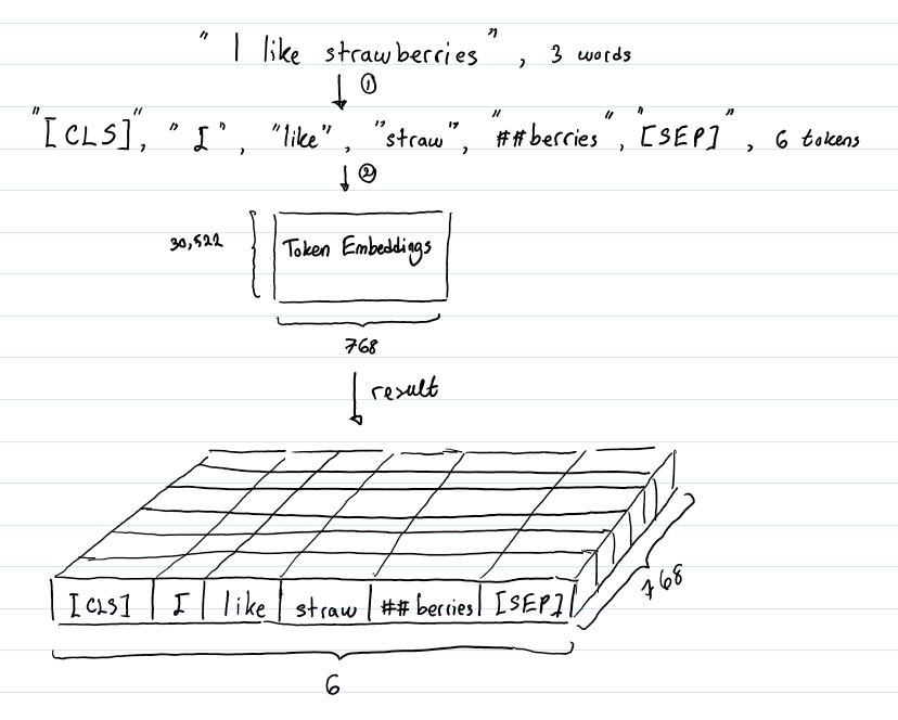
The challenge has provided us with a file named Lost in Hyperspace.zip. This file contains a .npz file named token_embeddings.npz

If you have never heard of an ‘npz’ file, you are not the only one. I have no idea how to solve this challenge 🙂. Joking aside, an npz file is used for NumPy, a python library used for linear algebra (it does a lot more, but we are not interested in that).

Our affected file contains precomputed embeddings for tokens. Let’s start from the basics, while tokens are the textual units, embeddings are high-dimensional vector representations of these tokens. Our file contains vectors that have already been generated.

Understanding the process 🔎

Let’s create a simple script to list all the arrays on the file

import numpy as np

data = np.load('token_embeddings.npz')

print(list(data.keys()))

The result will be: ['tokens', 'embeddings']

Now that we know the names of the two arrays, let’s extract them

import numpy as np

data = np.load('token_embeddings.npz')
tokens = data['tokens']
embeddings = data['embeddings']

So how do we solve this challenge ❓

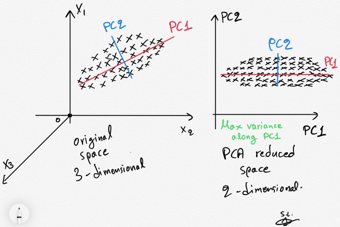
Embeddings are vector representations in a high-dimensional space. Now to display them (and thus obtain the 🚩) we must reduce the size of these vectors using PCA.

PCA (Principal Component Analysis) is a technique that reduces the dimensionality of the data while maintaining as much variance as possible in the original data.

Import it from the sklearn.decomposition library

So now this is the code:

import numpy as np
from sklearn.decomposition import PCA

data = np.load('token_embeddings.npz')
tokens = data['tokens']
embeddings = data['embeddings']

pca = PCA(n_components=2)
re_embeddings = pca.fit_transform(embeddings)

pca = PCA(n_components=2)

We are transforming embeddings into a two-dimensional plane.

re_embeddings = pca.fit_transform(embeddings)

• fit method computes the components from the data by determining the axes. It learns the structure of the data
• transform reduces the dimensionality by providing new coordinates.

Importing matplotlib 🧪

To create a scatter graph of embeddings reduced to two dimensions we can use matplotlib

import numpy as np
import matplotlib.pyplot as plt
from sklearn.decomposition import PCA

data = np.load('token_embeddings.npz')
tokens = data['tokens']
embeddings = data['embeddings']

pca = PCA(n_components=2)
re_embeddings = pca.fit_transform(embeddings)

plt.figure(figsize=(20, 12))
plt.scatter(re_embeddings[:, 0], re_embeddings[:, 1], alpha=0.6, s=100, edgecolor='k')
for i, token in enumerate(tokens):
    plt.text(re_embeddings[i, 0] + 0.02, re_embeddings[i, 1], str(token), fontsize=12, fontweight='bold')

plt.title('token embeddings PCA:')
plt.xlabel('1 principal component')
plt.ylabel('2 principal component')
plt.grid(False)
plt.show()

• plt.figure(figsize=(20, 12)) specifies the size of the figure in inches (20x12)
• plt.scatter(re_embeddings[:, 0], re_embeddings[:, 1] we select the first and second components of the reduced embeddings
• alpha=0.6 point transparency
• s=100 point dimension
• edgecolor='k' point colour (black)

And all other lines concern the graph, which is no interest to us.

Output 🖥️

The output is this:

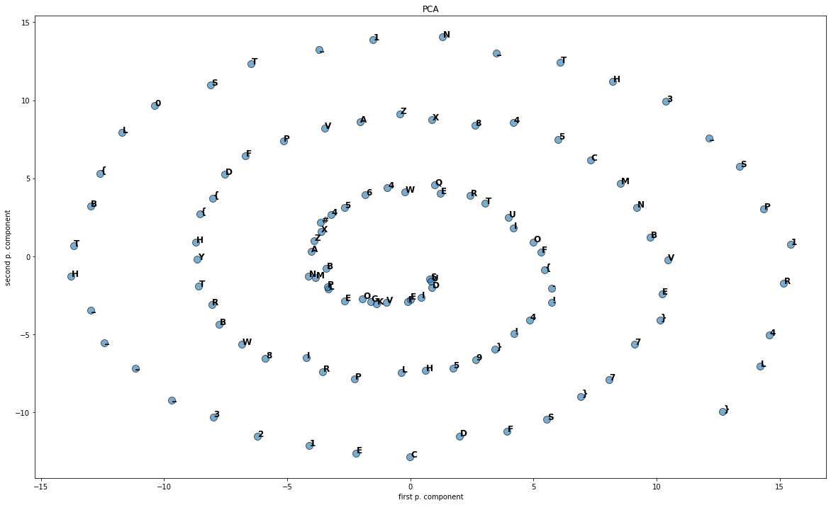
As you can see, the flag is this:

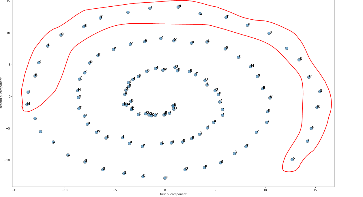
Flag: HTB{L0ST_1N_TH3_SP1R4L}